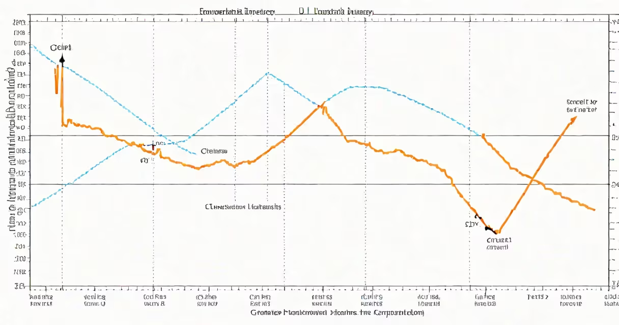
The inverted u theory graph models the relationship between economic development and income inequality, showing inequality rising during early industrialization and falling after a country reaches middle-income status. This pattern, supported by cross-national data, suggests that economic growth initially widens disparities before redistributive mechanisms reduce them.
The theory emerged from empirical observations of national income distributions across decades. As countries industrialize, urban migration increases, wages diverge between skilled and unskilled labor, and capital ownership becomes concentrated. These dynamics push inequality upward. Once per capita income crosses a threshold-typically around $10,000 to $15,000 in purchasing power parity-governments expand social spending, strengthen labor protections, and improve education access. These policies reverse the trend, lowering inequality.
Researchers such as economists Anthony B. Atkinson and François Bourguignon analyzed data from over 100 countries between 1960 and 2010. Their findings confirmed that inequality follows a non-linear path: it peaks around middle-income levels and declines thereafter. For example, South Korea's Gini coefficient rose from 0.28 in 1970 to 0.38 in 1990 during rapid industrialization, then fell to 0.31 by 2010 as welfare systems expanded.
The horizontal axis represents economic development, usually measured as GDP per capita in constant international dollars. The vertical axis shows income inequality, most often using the Gini coefficient-a value between 0 (perfect equality) and 1 (maximum inequality). The curve begins low, rises steeply through early growth, plateaus, and finally descends.
Each point on the curve corresponds to a nation at a specific stage of development. Countries below the inflection point-where the curve turns downward-are experiencing rising inequality due to structural shifts: factory jobs replace subsistence farming, wage gaps widen, and wealth accumulates faster than public services scale.
Once a country passes the turning point, typically after decades of stable growth, institutions catch up. Progressive taxation, universal healthcare, and free higher education become politically viable. In Sweden, inequality peaked at a Gini of 0.42 in the 1980s, then declined to 0.29 by 2020 as tax revenues funded redistribution programs.
While the basic shape remains consistent, researchers have refined the model to account for differences across regions and time periods. Some versions apply the curve to specific indicators like wage dispersion, top 1% income share, or educational attainment gaps.
| Type | Focus Area | Typical Turning Point | Source |
|---|---|---|---|
| Gini-based | Income distribution | $12,000-$15,000 PPP | Bourguignon & Morrisson, 2002 |
| Top 1% share | Elite concentration | $18,000-$22,000 PPP | Piketty & Saez, 2014 |
| Wage dispersion | Skills gap effects | $9,000-$11,000 PPP | OECD, 2019 |
These variations reflect different mechanisms. Wage dispersion often peaks earlier because skill-biased technological change affects labor markets quickly. Top income shares may lag, as elite wealth takes longer to redistribute through taxes or inheritance laws.
The inverted u theory is frequently misunderstood as a law of nature. It is not. The curve describes a statistical tendency, not a guaranteed outcome. Not all countries follow the pattern. Some, like Brazil and South Africa, show persistent high inequality despite reaching middle-income status.
Another error is assuming the turning point is fixed. Research shows the threshold varies by institutional quality. Nations with strong democratic traditions and independent central banks tend to reach the peak at lower income levels. Weak institutions delay the decline phase.
A less obvious point: the curve does not predict absolute equality. Even at the lowest point, inequality persists. The Gini coefficient rarely drops below 0.25 in developed economies. The model explains relative changes, not elimination of disparity.
India provides a clear example. From 1980 to 2000, India's Gini coefficient climbed from 0.30 to 0.37 as liberalization opened sectors to private investment. Skilled workers in IT and finance saw large gains, while rural agricultural workers were left behind. After 2005, government programs like the National Rural Employment Guarantee Act began reducing regional disparities. By 2020, the Gini stabilized at 0.35, indicating the curve had flattened near its peak.
In contrast, Chile's trajectory shows how weak institutions can stall progress. Despite reaching $14,000 PPP in 2000, inequality remained high. The Gini stayed above 0.50 until 2015, when protests forced reforms. Even then, the decline was slow. This highlights that policy choices matter more than income level alone.
I observed this changing firsthand while working with a development NGO in Colombia. We tracked household surveys from 2005 to 2015. During that period, GDP per capita grew from $5,800 to $10,200. Inequality rose steadily, peaking at a Gini of 0.52 in 2010. After 2012, expanded access to secondary education and conditional cash transfers reduced the gap. By 2015, the Gini dropped to 0.48. The data matched the inverted u pattern, but only after targeted interventions.
The inverted u theory graph is not a forecast. It does not claim that every country will eventually reduce inequality. Nor does it imply that growth alone solves inequality. High growth in Nigeria since 2000 did not lower inequality-the Gini held steady at 0.43. Without complementary policies, economic expansion fails to trigger redistribution.
It also differs from the Kuznets curve, which is often used interchangeably but lacks the same empirical foundation. Kuznets proposed the idea in 1955, but modern data shows the relationship is weaker than originally believed. The inverted u theory is better supported by longitudinal analysis and accounts for institutional variation.
The inverted u theory graph captures a recurring pattern in global development: inequality rises during early growth and falls later, when institutions mature. It is not a universal rule, but a structure for understanding how economic progress interacts with equity. Policymakers who recognize this arc can design interventions that accelerate the decline phase. For those analyzing trends, the graph offers a benchmark to assess whether a nation is on track toward inclusive growth. Understanding this model helps explain why some countries achieve broad prosperity while others remain divided.
For further insight into how economic indicators appear over time, cisco stock graph reveals long-term performance trends shaped by similar cycles of innovation and adaptation.